Lab 3 - Unsupervised Classification

Goal and Background

The main goal of this lab exercise was to develop an understanding of the use of unsupervised classification methods to extract information about surface features from remotely sensed images.  The first part of this lab was focused on learning about inputs and configuration requirements necessary to run the unsupervised classifier.  The second part of this lab was focused on taking the spectral classes created by the classifier and recoding them into useful thematic information about land-use/land-cover (LULC).

Methods

Part 1: Experimenting with unsupervised ISODATA classification algorithm

To start off this lab, we were given an image of Eau Claire and Chippewa counties from Landsat ETM+ captured in June of 2000.  We used this image to run a Iterative self-organizing data analysis technique (ISODATA) by using the Unsupervised Classification tool under Raster>Unsupervised>Unsupervised Classification.  With the Unsupervised Classification tool window open, the input image of Eau Claire and Chippewa counties was put in and the output image was saved to the correct folder.  Next, the ISODATA radio button was checked under the "Method" section and the number of classes was changed to be 10.  The default parameters for "Initializing Options" as well as "Color Scheme Options" was selected followed by the default value for the convergence threshold before changing the "Maximum Iterations" to 250.  After all the correct inputs were finalized, the model was run and the resulting image was brought into the viewer.  With the classified image open in the viewer, the attribute table was opened and the viewer was synced to Google Earth to help in identifying the features to be classified.  By changing the color of each class to a brighter, more identifiable color and comparing what features are that color we created 5 distinct LULC classes.  These classes were water (blue), forest (dark green), agriculture (pink), urban/built-up (red), and bare soil (sienna). 

Part 2:  Improving the accuracy of unsupervised classification

Part 2 of this lab was similar to part 1 as the same ISODATA unsupervised classification scheme was used but with slightly different input parameters compared to part 1.  The only input parameters that were different in this iteration compared to the first was a Convergence Threshold of 0.92 as compared to the 0.95 used in part 1 and a maximum number of classes of 20 compared to the 10 classes created in part 1.  Once these parameters were changed, the tool was run and the output image was brought into a viewer.  Just as in part 1, the attribute table was opened and all 20 of the classes were labeled as belong to one of the five classes; water, forest, agriculture, urban/built-up, or bare soil.  Once this was done, the Raster Attribute Editor and the Column Properties window was used to better order the data in the attribute table for easier analysis.  Once this was done, the next step was to create a map using the 20 classifications but to do this those 20 classifications needed to be cut down to 5.  To do this, the Recode tool was used under Raster<Thematic<Recode.  Using the Recode tool and the Thematic Recode window, the 20 classes were condensed into 5 classes, one for each of the LULC classes.  Again, column properties were edited to make analysis easier and finally the image was exported into Arcmap where a map was created to represent the various LULC classes for Eau Claire and Chippewa counties.

Results

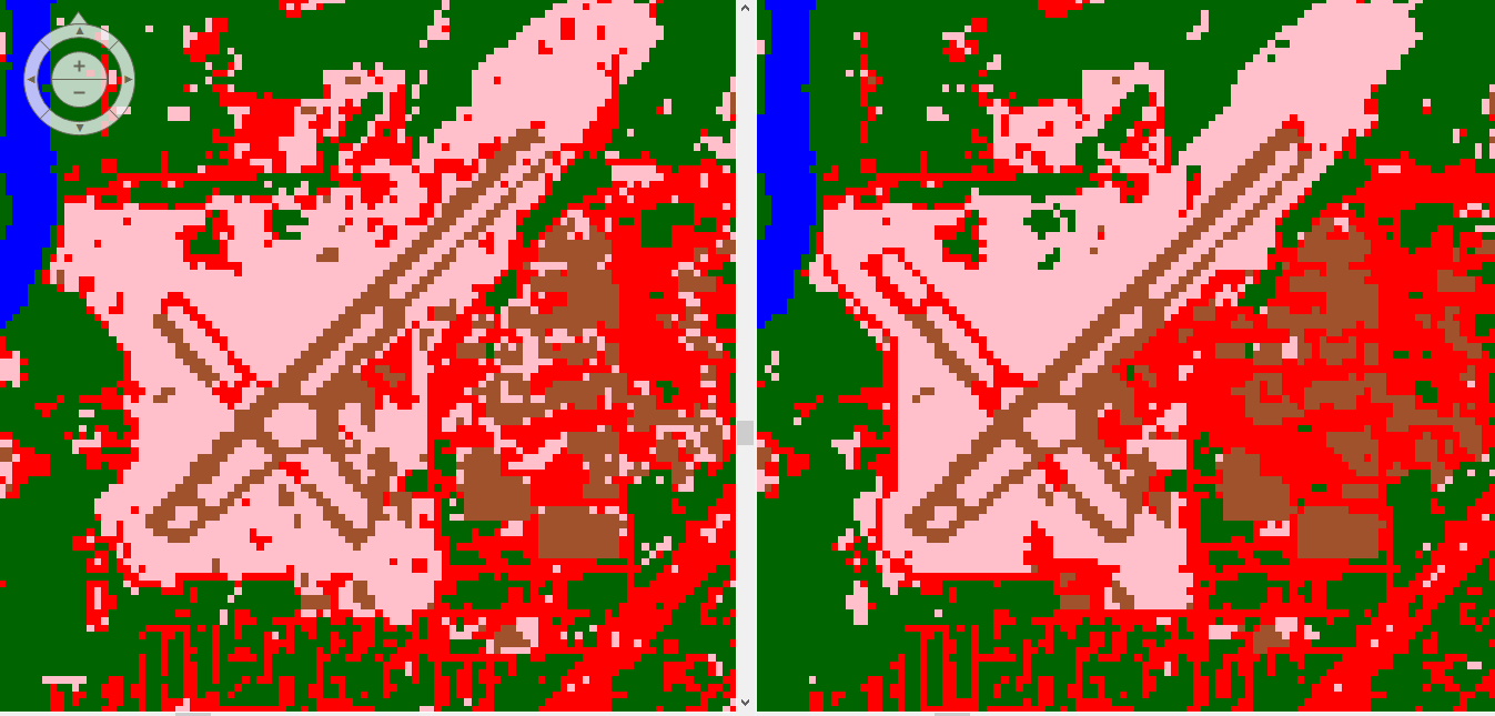
Figure 1. - Difference between 10 classes (left) and 20 classes (right) showing the higher accuracy present with a higher number of classes.

Figure 2. - Final attribute table of five classes once Recode tool had been used.

Figure 3. - Final map showing various LULC of Eau Claire and Chippewa counties.

Sources

 Landsat satellite image is from Earth Resources Observation and Science Center, United States Geological Survey. 

Lab 2 - Radiometric and Atmospheric Correction

Goal and Background

The goal of this lab was to develop an understanding and experience in the atmospheric correction of images using both relative and absolute atmospheric correction models.  These models included Empirical Line Calibration (ELC), Image Based Dark Object Subtraction (DOS), and Multi-Date Image Normalization.  

Methods

Part 1: Absolute atmospheric correcting using empirical line calibration

For part 1, ELC was calculated with the following equation, where DN was the band(s) to be corrected, M was a multiplicative term for the brightness value, and L was an additive term.

Using the Raster>Hyperspectral>Spectral Analysis Workstation tool as well as the Atmospheric Adjustment tool, we were able to collect points on vegetation, concrete, and other surface features and compare their spectral profiles to those within the ASTER and USGS V4 spectral libraries.  In the Spectral Analysis Workstation we then ran the Preprocess>Atmospheric Adjustment model to create an output atmospherically corrected image that used the ELC equation and information collected above.  This image was then compared to the original uncorrected image to judge how well this correction method works.

Part 2: Absolute atmospheric correction using enhanced image based Dark object subtraction

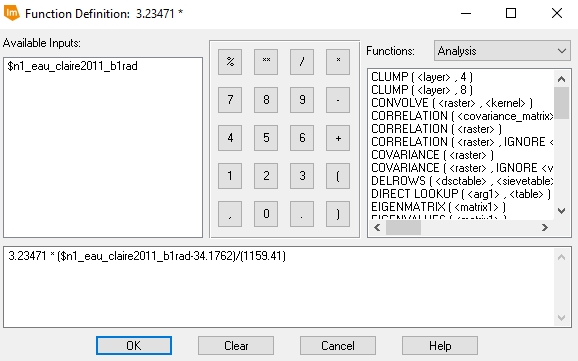
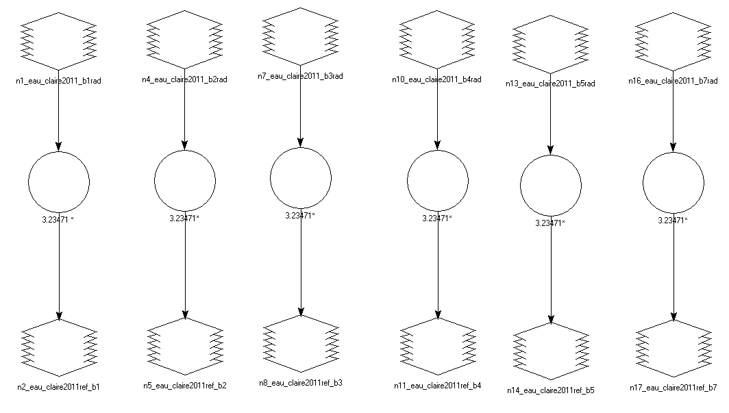
The first step in atmospherically correcting an image using the DOS method was to create a model that converted the satellite image to at-satellite spectral radiance for bands 1-5 and 7 simultaneously.  To do this, the equation below was used using data collected form the metadata text file associated with the individual band images.

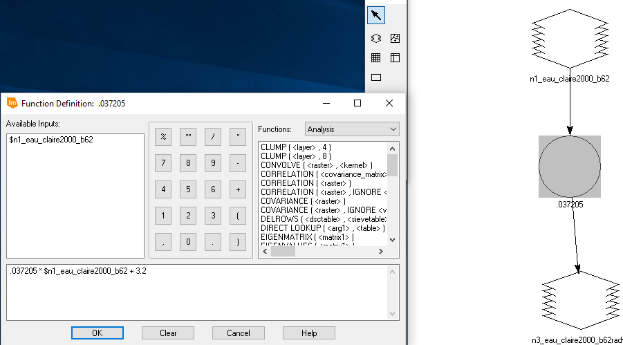
Next, the at-satellite spectral radiance images for each individual band that were the results of the model were then converted to true surface reflectance using the equation below with values calculated from the histograms of the radiance images, distance between the Earth and Sun calculated from an Earth-Sun distance table, the Sun zenith angle calculated from the image metadata file, and the Esun value from a table on Landsat TM.

Once both models were completed, true surface reflectance images for each band were layer stacked and then spectral profiles of a variety of features were collected to compare to the original uncorrected image.

Part 3: Relative atmospheric correction using multi-date image normalization

The first step in multi-date image normalization was to collect points off of pseudo-invariant features from base image and subsequent image.  This was done by using the same Spectral Profile tool used elsewhere in the lab.  The tabular data from these spectral profiles were then copied into Excel where scatter plots were created and regression equations were calculated. Using the values in the regression equations, a model was created to correct each individual band to create individual images of each band that were corrected.  To do this, the following equation was used.

Once the model was run, the resulting corrected band images were layer stacked to create a false color image that was then compared to the original image.

Results

Example model and equation for conversion of image to at-satellite spectral radiance image

Example of model and equation for at satellite spectral radiance to true surface reflectance

Chicago 2000 Image Spectral Profiles

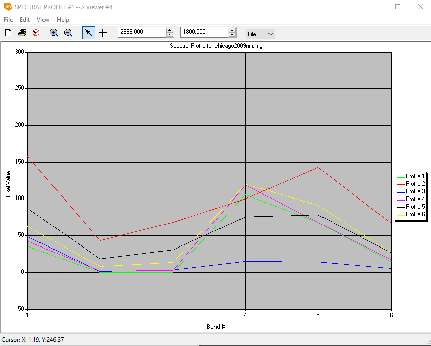
Chicago 2009 Image Spectral Profiles

Scatter Plots of Mean Pixel Values per Band

Spectral Profiles of Chicago 2000 and Chicago 2009 After Relative Correction

Sources

 Landsat satellite image is from Earth Resources Observation and Science Center, United States Geological Survey. Spectral signatures are from the respective spectral libraries consulted - ASTER, USGS V4

Lab 1 - Thermal Remote Sensing

Goal and Background

The goal of this lab was to introduce us students to the principles of extracting land surface temperatures from a variety of Earth features using the thermal bands of different Landsat satellites.  This lab was also designed so that we would develop an understanding of surface temperature variations over time and space, developing models to derive surface temperature, and combining simple models to form more complex models.

Methods

Part 1: Visual identification of relative variations in land surface temperature

Part 1 of this lab was all about an introductory into viewing remotely sensed thermal images.  To do this, different thermal images from Landsat ETM+ band 6, both high gain and low gain, were provided so that we could compare the tonal differences between the two different images.

Part 2: Calculation of land surface temperature from ETM+ image

Part 2 of this lab was all about developing two separate and simple models to first take the provided ETM+ image and convert it into an at-satellite radiance image.  To do this, a simple model with the equation Grescale * DN + Brescale was used with the Grescale and Brescale being calculated from information in the metadata of the image.  Once the model was run and the at-satellite radiance image obtained, a second model was created to covert this image into a blackbody surface image that showed surface temperature in degrees Kelvin.  This model was run with the provided k1 and k2 calibration constants.  The resulting image from this second model was brought into Arcmap so that the identification tool could be used to check the temperature of a variety of surface features.

Part 3: Calculation of land surface temperature from TM image

Part 3 of this lab focused on calculating surface temperatures from a TM image using the same equations from part 2 but instead of two separate models, a single model was used.  Just like in part 2, the Grescale and Brescale were calculated using data within the image metadata and then the provided k1 and k2 constants were used.  The difference in this model was making sure to check the "Temporary Raster Only" radio button in the output at-satellite radiance image so that no image would be saved and the model could just use that temporary image to finish the conversion to a land surface temperature image.  The resulting image showed surface temperatures in degrees Kelvin for the Eau Claire area and was used to answer some questions about specific land features temperatures.

Part 4: Calculation of land surface temperature from Landsat 8 image

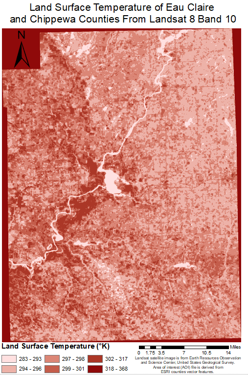
Part 4 of this lab was nearly identical to part 3, but instead used and image from Landsat 8 rather than TM.  The only difference that occurred because of this difference in which satellite was used was that the k1 and k2 constants were located in the metadata rather than provided by the instructor.  The same model from part 3 was run on the image after it had been subsetted to just Eau Claire and Chippewa counties.  The resulting surface temperature image was then brought into Arcmap where it was cleaned up and labeled into a standalone map.

Results

Example of model from part 2: conversion to an at-satellite radiance image

Final map of Landsat 8 thermal image

Sources

 Landsat satellite image is from Earth Resources Observation and Science Center, United States Geological Survey

Area of interest (AOI) file is derived from ESRI counties vector features.